The Raspberry Pis
For our servers and clients, we used 8 raspberry pi 3B+ running a modified Raspbian image. Each of these can be purchased for under $50. As they run Linux, they are able to run all of the different congestion control algorithms (specially, we are interested in BBR).
We provide information on the steps we took to recompile the Kernel, as well as performance measurements for the Pis.
The Router
The router is an ubuntu desktop with 3 nic cards. One card is used for the normal ‘wide area network’, and the other two cards are used to route between the two raspberry pi subnets. This is done using netplan on ubuntu, and editing the dhcpd.conf to set up static ip addresses. Also, the host files for each machine are edited to make tests more convenient.
Adding congestion control protocols
The linux kernel comes with a number of different congestion control algorithms. To test new congestion control methods we to be able to:
- Dynamically select new protocols
- Recompile and install new protocols
Running an Experiment
A typical experiment involves setting the congestion control protocols for each raspberry pi, setting the bandwidth and latency parameters for the router, and running a packet capture on each sender and client to monitor the flow.
Parsing and Plotting Captures
The start_trial script described here copies 8 packet capture (pcap) files to a local ‘Results’ directory. This page describes the tools used to parse these captures and create plots of the goodput (throughput seen by the receiver), the round trip times (for the sender) and the packets in flight (for the sender).
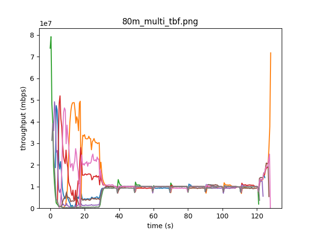
The goal is to parse each experiment, the 8 pcap files, into 8 csv files, and then to create plot like this:
Improving the Experiment setup
Being able to quickly run and rerun experiments is vital in ensuring that the tweaks we make to our testbed are having the effects that we expect. Specifically, we needed to be able to:
Setup the router with the correct parameters
Increasing or decreasing the bandwidth, latency, buffer size etc.
Orchestrate the raspberry pi startup
This involves starting up
Nflows per raspberry pi, and measuring their performance over the course of the experiment session.And, for each raspberry pi, needed to start a packet capture to analyze the results post experiment.
Poll the router as the experiment progresses
This allows us to see the ‘ground truth’ for how many packets are in flight or dropped. (Currently, we only keep track of the router queue size).
Pull in all of the captures to the ‘router’
Parse the captures into CSV files and create consistent plots
By wrapping all of these procedures in a single script, we are able to quickly change configurations and create plots in an identical manner. The reproducibility of this setup is key in allowing us to compare results across different configurations in a consistent manner.